In my previous tutorial, I gave a brief idea about the fundamentals of digital signal processing. Now we are going to take a step further in this direction. To do the processing part we first need to understand discrete-time signals, classification and their operations. In this tutorial major emphasis will be given on Discrete-time signals and discrete-time systems.
What we are going to learn in this tutorial :-
- Sampling
- {Discrete-time Signals
- {C}{ Classification of Discrete-time signals
- Transformation of Discrete-time signals
- Sampling
- First we need to understand what is a Sampling process? Why do we need sampling? The answer to the first question is that Sampling is a process of breakage of continuous signal to discrete signal. In a layman definition the output of system is recorded at different intervals of time, these intervals of time may not necessarily be uniform but in this series of tutorials we will limit our discussion to only Uniform-Sampling.
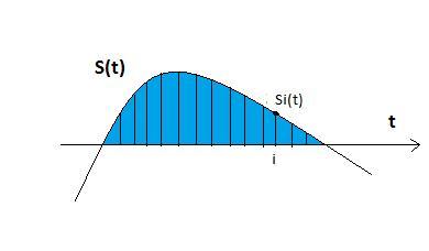
- In the above picture shown the continuous signal S(t) is being sampled at different moments of time, let the ith value be Si(t) then the set of values of Si(t) from i=0 to n are called the samples of S(t). Time interval between two consecutive sampling intervals is called Sampling period or Sample interval. If the time interval between two consecutive sampling intervals is uniform and equals to T,

fs= 1/T , where fs is the sampling frequency.
- Discrete-time Sinusoids :-
- Discrete-time sinusoids are a very important type of signal which is to be studied under Digital Signal Processing. So, since now we have a brief idea about sampling, we will be discussing about those signals and then we will get to the Sampling Theorem. A discrete-time sinusoidal signal may be expressed as,
x(n)= Acos(?0n + Ø) , -? < n < +?
- Where n is an integer, ?0 is the angular frequency and is also equal to 2?f0, where f0 is the frequency and Ø is the phase of the signal. Discrete-time sinusoids are periodic only if the frequency of the signal is a rational number. We need to prove this statement,
x(n+N) = x(n)
or, cos[2?f0(n+N) + Ø] = cos[2?f0(n) + Ø]
or, 2?f0N=2k?
or, f0 =k/N
- Also, there is one more interesting properties of Discrete-time sinusoids. Discrete-time signals whose frequencies are separated by an integral multiple of 2? are identical. Let there be another signal x2(t) which differs from the previous signal with a phase difference of 2?, then the x2(t) can be written as,
x2(t) = Acos[(?0 +2?)n + Ø]= Acos(?0 n+2?n + Ø)= Acos(?0n + Ø)
- which is equal to the former signal x(t). This can be interpreted as if a signal has a frequency |?| > ?. Then this signal can be said to be identical to another signal obtained from a signal with frequency |?| < ?. Thus we can say that,
|?|? ?
Or, |f| ? ½
- All the frequencies in the above specified range are regarded as unique and all the other frequencies are said to be ‘aliases’. Now it’s high time to answer the second question regarding the need of sampling, the fact that most of the signals in nature are analog caters to the need of sampling and since in my previous tutorial I have made clear benefits of Digital Signal Processing over Analog Signal Processing, to obtain Discrete-time signals we have to do sampling of the Analog signals. Now let xa(t) be an analog signal and xa(t) with frequency F sampled periodically to obtain xa(nT) at a frequency 1/T. Then,
Ananlog signal, xa(t) = A cos(2?Ft + Ø)
Discrete-time signal, xa(nT) = A cos(2?FnT + Ø)
Or, xa(nT) = A cos(2?Fn/Fs + Ø)
- As we have discussed above in the discrete-time sinusoids |f| ? ½, Thus we conclude that,
|F/Fs| ? ½
Or, |F| ? Fs/2
Thus we can clearly see that if the max. frequency of the signal is Fmax then the sampling frequency, Fs must be greater than twice Fmax. This is also known as Nyquist Rate of sampling. This is always to be remembered that Fs must be twice the “max.” frequency component of the signal not just any frequency of the signal otherwise it will induce attenuation and signal distortion.
Sampling Theorem: If the highest frequency contained in any analog signal xa(t) is Fmax=B and sampling is done at a frequency Fs > 2B, then xa(t) can be exactly recovered from its samples using the interpolation function,
G(t) = sin (2?Bt)/2?Bt
Thus,